Virasoro Representations

Goal

The previous page introduced the Virasoro algebra,

$$[L_m,L_n] = (m-n)L_{m+n} + \frac{c}{12}m(m^2-1)\delta_{m+n,0},$$

with an independent antiholomorphic copy generated by $\bar L_n$. This page explains how a two-dimensional CFT Hilbert space is built from representations of this algebra.

The main idea is beautifully close to the representation theory of the finite-dimensional conformal algebra, but much stronger. A local primary operator creates a highest-weight state. Negative Virasoro modes create descendants. The resulting tower is a Verma module. Sometimes the tower contains a null state, and quotienting by the null submodule gives a smaller irreducible representation. In correlation functions, null states become differential equations. These are the BPZ equations, one of the classic reasons two-dimensional CFT is exactly solvable.

For AdS/CFT, this page has three immediate uses. First, in AdS$_3$/CFT$_2$, Virasoro descendants of the vacuum are boundary gravitons. Second, Virasoro conformal blocks organize two-dimensional CFT correlators far more finely than global conformal blocks. Third, in worldsheet string theory, the physical state conditions are Virasoro constraints.

From local operators to highest-weight states

In radial quantization, a local operator inserted at the origin creates a state:

$$|\mathcal O\rangle=\mathcal O(0,0)|0\rangle.$$

For a primary operator $\phi(z,\bar z)$ with weights $(h,\bar h)$, the stress-tensor OPEs are

$$T(z)\phi(w,\bar w) \sim \frac{h\phi(w,\bar w)}{(z-w)^2} + \frac{\partial\phi(w,\bar w)}{z-w},$$

and

$$\bar T(\bar z)\phi(w,\bar w) \sim \frac{\bar h\phi(w,\bar w)}{(\bar z-\bar w)^2} + \frac{\bar\partial\phi(w,\bar w)}{\bar z-\bar w}.$$

Using

$$L_n=\frac{1}{2\pi i}\oint_0 dz\,z^{n+1}T(z), \qquad \bar L_n=\frac{1}{2\pi i}\oint_0 d\bar z\,\bar z^{n+1}\bar T(\bar z),$$

the state created by $\phi$ obeys

$$L_0|h,\bar h\rangle=h|h,\bar h\rangle, \qquad \bar L_0|h,\bar h\rangle=\bar h|h,\bar h\rangle,$$

and

$$L_n|h,\bar h\rangle=0, \qquad \bar L_n|h,\bar h\rangle=0, \qquad n>0.$$

This is the two-dimensional version of a highest-weight condition. The positive modes annihilate the primary state. The negative modes generate descendants.

The scaling dimension and spin are

$$\Delta=h+\bar h, \qquad s=h-\bar h.$$

The full representation of the local conformal algebra is usually a tensor product of a holomorphic Virasoro representation and an antiholomorphic Virasoro representation:

$$\mathcal H_{h,\bar h} \simeq \mathcal H_h\otimes \bar{\mathcal H}_{\bar h}.$$

The holomorphic and antiholomorphic sectors commute:

$$[L_m,\bar L_n]=0.$$

So one can usually study the holomorphic representation first and then take the product with the barred copy.

Highest-weight representations

A holomorphic highest-weight state $|h\rangle$ is defined by

$$L_0|h\rangle=h|h\rangle, \qquad L_n|h\rangle=0\quad(n>0).$$

The number $h$ is the holomorphic conformal weight. The central charge $c$ is fixed by the CFT, so the representation is labeled by

$$(c,h).$$

The negative modes

$$L_{-1},L_{-2},L_{-3},\ldots$$

act as raising operators for $L_0$. Indeed, from

$$[L_0,L_n]=-nL_n,$$

we get

$$L_0\bigl(L_{-n}|h\rangle\bigr) = (h+n)L_{-n}|h\rangle.$$

Thus $L_{-n}$ raises the $L_0$ eigenvalue by $n$.

A general descendant state has the form

$$L_{-n_1}L_{-n_2}\cdots L_{-n_k}|h\rangle, \qquad n_i>0.$$

Using the Virasoro commutation relations, one may order the modes as

$$n_1\ge n_2\ge\cdots\ge n_k>0.$$

The level of this descendant is

$$N=n_1+n_2+\cdots+n_k.$$

It has $L_0$ eigenvalue

$$h+N.$$

The level is the holomorphic descendant number. In radial quantization it is the excitation energy above the primary state.

Verma modules

The Verma module $M(c,h)$ is the vector space generated by acting freely with all negative Virasoro modes on $|h\rangle$:

$$M(c,h) = \operatorname{span}\left\{ L_{-n_1}L_{-n_2}\cdots L_{-n_k}|h\rangle \;\middle|\; n_1\ge n_2\ge\cdots\ge n_k>0 \right\}.$$

The first few levels are

$$N=0: \qquad |h\rangle,$$ $$N=1: \qquad L_{-1}|h\rangle,$$ $$N=2: \qquad L_{-2}|h\rangle, \quad L_{-1}^2|h\rangle,$$ $$N=3: \qquad L_{-3}|h\rangle, \quad L_{-2}L_{-1}|h\rangle, \quad L_{-1}^3|h\rangle.$$

At level $N$, the independent ordered monomials correspond to partitions of $N$. Therefore the number of states at level $N$ in a generic Verma module is

$$p(N),$$

where $p(N)$ is the partition number. The generating function is

$$\sum_{N=0}^{\infty}p(N)q^N = \prod_{n=1}^{\infty}\frac{1}{1-q^n}.$$

The holomorphic character of a generic Verma module is therefore

$$\boxed{ \chi_{M(c,h)}(q) = \operatorname{Tr}_{M(c,h)} q^{L_0-c/24} = q^{h-c/24}\prod_{n=1}^{\infty}\frac{1}{1-q^n}. }$$

The factor $q^{-c/24}$ is the cylinder Casimir shift. It appears because the Hamiltonian on the cylinder is not $L_0$ but $L_0-c/24$ in the holomorphic sector.

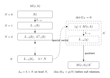
A generic Verma module $M(c,h)$ is freely generated by negative Virasoro modes. At special values $h=h_{r,s}(c)$, a null singular vector $|\chi\rangle$ appears at level $N=rs$. It generates a submodule $\mathcal N$. The irreducible representation is the quotient $\mathcal L(c,h)=M(c,h)/\mathcal N$.

Descendants as local operators

The state-operator map turns every descendant state into a descendant operator. The simplest examples are

$$L_{-1}|h,\bar h\rangle \quad\longleftrightarrow\quad \partial\phi(0,0),$$

and

$$\bar L_{-1}|h,\bar h\rangle \quad\longleftrightarrow\quad \bar\partial\phi(0,0).$$

Higher descendants are less simply expressed as ordinary derivatives because modes such as $L_{-2}$ involve the stress tensor. A useful operator definition is

$$(L_{-n}\phi)(z) = \frac{1}{2\pi i}\oint_z dw\,(w-z)^{1-n}T(w)\phi(z), \qquad n\ge 1.$$

For $n=1$, the $T\phi$ OPE gives

$$(L_{-1}\phi)(z)=\partial\phi(z).$$

For $n\ge 2$, $L_{-n}\phi$ is a genuinely Virasoro descendant. It is a local operator in the same Virasoro family as $\phi$.

A Virasoro family is much larger than a global conformal family. The global family uses only $L_{-1}$ descendants, while the Virasoro family uses every $L_{-n}$ with $n>0$. This is why Virasoro conformal blocks resum infinitely many global conformal blocks.

Inner product and the Shapovalov form

In a unitary CFT, radial quantization gives the adjoint relation

$$L_n^\dagger=L_{-n}.$$

Thus inner products of descendants are determined by the Virasoro algebra. For example,

$$\langle h|L_1L_{-1}|h\rangle = \langle h|[L_1,L_{-1}]|h\rangle =2\langle h|L_0|h\rangle =2h\langle h|h\rangle.$$

If we normalize $\langle h|h\rangle=1$, then

$$\|L_{-1}|h\rangle\|^2=2h.$$

Unitarity therefore requires

$$h\ge 0.$$

At level $2$, use the basis

$$\left\{L_{-2}|h\rangle,\;L_{-1}^2|h\rangle\right\}.$$

The Gram matrix is

$$G^{(2)}= \begin{pmatrix} \langle h|L_2L_{-2}|h\rangle & \langle h|L_2L_{-1}^2|h\rangle \\ \langle h|L_1^2L_{-2}|h\rangle & \langle h|L_1^2L_{-1}^2|h\rangle \end{pmatrix}.$$

A direct Virasoro-algebra computation gives

$$\boxed{ G^{(2)}= \begin{pmatrix} 4h+\frac{c}{2} & 6h \\ 6h & 4h(2h+1) \end{pmatrix}. }$$

For unitarity, every Gram matrix at every level must be positive semidefinite. This is a strong condition. It is the two-dimensional analogue of higher-dimensional unitarity bounds, but because there are infinitely many Virasoro descendants, the constraints are much sharper.

The determinant at level $2$ is

$$\det G^{(2)} = 2h\left(16h^2+(2c-10)h+c\right).$$

When such determinants vanish, a null state appears.

Null states and singular vectors

A null state is a nonzero state with zero norm that is orthogonal to every state in the module. A singular vector is a descendant state that is itself highest-weight:

$$L_n|\chi\rangle=0, \qquad n>0.$$

In a highest-weight module, null states that matter for representation theory are singular vectors. They generate submodules.

For example, suppose a level-$2$ singular vector has the form

$$|\chi\rangle = \left(L_{-2}+aL_{-1}^2\right)|h\rangle.$$

Demanding $L_1|\chi\rangle=0$ gives

$$3+a(4h+2)=0,$$

so

$$a=-\frac{3}{2(2h+1)}.$$

Demanding $L_2|\chi\rangle=0$ then gives

$$4h+\frac{c}{2}+6ah=0.$$

Equivalently,

$$\boxed{ |\chi\rangle = \left( L_{-2}-\frac{3}{2(2h+1)}L_{-1}^2 \right)|h\rangle }$$

is null when

$$\boxed{ 16h^2+(2c-10)h+c=0. }$$

This is the nontrivial level-$2$ factor of the determinant. The other level-$2$ zero occurs at $h=0$, where the descendant $L_{-1}|0\rangle$ is already null in the vacuum representation.

If the theory is unitary, null states have zero norm and decouple from all physical correlation functions. The irreducible representation is obtained by quotienting out the submodule generated by the null state:

$$\mathcal L(c,h)=M(c,h)/\mathcal N.$$

This quotient is not a technicality. It changes the spectrum of descendants and makes the character smaller.

The vacuum module

The identity operator creates the vacuum:

$$|0\rangle=\mathbf 1(0)|0\rangle.$$

The vacuum is invariant under the global conformal group:

$$L_{-1}|0\rangle=L_0|0\rangle=L_1|0\rangle=0.$$

The condition

$$L_{-1}|0\rangle=0$$

says that translating the identity operator gives zero:

$$\partial\mathbf 1=0.$$

Thus the vacuum representation is not the generic Verma module $M(c,0)$. The level-$1$ state is removed. The first nontrivial holomorphic descendant is

$$L_{-2}|0\rangle,$$

which corresponds to the stress tensor:

$$T(0)|0\rangle=L_{-2}|0\rangle.$$

If there are no further null states, the vacuum character is

$$\boxed{ \chi_{\mathrm{vac}}(q) = q^{-c/24}\prod_{n=2}^{\infty}\frac{1}{1-q^n}. }$$

The product begins at $n=2$, not $n=1$, because $L_{-1}|0\rangle=0$.

In AdS$_3$/CFT$_2$, this character is the chiral counting of boundary gravitons. The vacuum descendants are created by $L_{-2},L_{-3},\ldots$, which are precisely the nontrivial asymptotic Virasoro excitations of the AdS$_3$ vacuum.

The Kac determinant

At level $N$, the Gram matrix of a Verma module is finite-dimensional, with dimension $p(N)$. Its determinant has a remarkable factorized form. One common parametrization is

$$c=13-6\left(t+\frac{1}{t}\right),$$

and

$$h_{r,s}(t) = \frac{(rt-s)^2-(t-1)^2}{4t}, \qquad r,s\in \mathbb Z_{>0}.$$

Then the Kac determinant is

$$\boxed{ \det G^{(N)}(c,h) = C_N \prod_{\substack{r,s\ge 1\\ rs\le N}} \left(h-h_{r,s}(c)\right)^{p(N-rs)}. }$$

Here $C_N$ is a nonzero normalization-dependent constant. The important physics is the zero locus:

$$\det G^{(N)}=0 \quad\Longleftrightarrow\quad h=h_{r,s}(c) \quad\text{for some }rs\le N.$$

At $h=h_{r,s}(c)$, a singular vector appears at level

$$N=rs.$$

This formula is the representation-theoretic backbone of the minimal models. It tells us exactly when a Verma module becomes reducible.

A caution: the symbols $r,s$ in $h_{r,s}$ are labels of Virasoro degenerate representations. They are not spacetime indices, and they have nothing to do with the spin $s=h-\bar h$.

Unitarity and the unitary minimal series

For $c\ge 1$, a highest-weight Virasoro representation is unitary when

$$h\ge 0.$$

For $0<c<1$, unitarity is dramatically more restrictive. The allowed central charges are discrete:

$$\boxed{ c_m=1-\frac{6}{m(m+1)}, \qquad m=3,4,5,\ldots }$$

The allowed weights are

$$\boxed{ h_{r,s}^{(m)} = \frac{\left((m+1)r-ms\right)^2-1}{4m(m+1)}, }$$

with

$$1\le r\le m-1, \qquad 1\le s\le m,$$

and the identification

$$h_{r,s}^{(m)}=h_{m-r,m+1-s}^{(m)}.$$

These are the unitary minimal models. They are rational CFTs: only finitely many irreducible Virasoro representations appear.

The first example is $m=3$, for which

$$c=\frac12.$$

The allowed weights are

$$h=0, \qquad h=\frac{1}{16}, \qquad h=\frac12.$$

These are the three chiral weights of the two-dimensional Ising CFT. In the diagonal Ising model, the primary fields are

$$\mathbf 1: (0,0), \qquad \sigma: \left(\frac{1}{16},\frac{1}{16}\right), \qquad \varepsilon: \left(\frac12,\frac12\right).$$

The fact that a lattice critical point can lead to a finite list of primary operators is one of the miracles of two-dimensional critical phenomena.

Null-state decoupling and BPZ equations

Null states are not merely representation-theoretic curiosities. They imply differential equations for correlation functions.

Let $\phi(z)$ be a primary field whose module contains the level-$2$ null state

$$\left( L_{-2}-aL_{-1}^2 \right)|h\rangle=0, \qquad a=\frac{3}{2(2h+1)}.$$

In the irreducible theory this means the descendant operator obeys

$$\left(L_{-2}\phi\right)(z) -a\partial_z^2\phi(z)=0.$$

Now insert this field into a correlator with other primary operators $\phi_i(z_i)$:

$$F(z;z_i) = \left\langle \phi(z)\prod_i\phi_i(z_i)\right\rangle.$$

Using the Ward identity to rewrite the $L_{-2}\phi$ insertion gives

$$\left\langle (L_{-2}\phi)(z)\prod_i\phi_i(z_i)\right\rangle = \sum_i \left[ \frac{h_i}{(z-z_i)^2} + \frac{1}{z-z_i}\partial_{z_i} \right]F(z;z_i).$$

Therefore the null-state condition gives the BPZ equation

$$\boxed{ \left[ \sum_i \left( \frac{h_i}{(z-z_i)^2} + \frac{1}{z-z_i}\partial_{z_i} \right) - \frac{3}{2(2h+1)}\partial_z^2 \right]F(z;z_i)=0. }$$

This is a second-order differential equation. For four-point functions it becomes an ordinary differential equation in the cross-ratio. Its solutions are Virasoro conformal blocks.

This is the BPZ mechanism:

$$\boxed{ \text{null vector} \quad\Longrightarrow\quad \text{decoupling equation} \quad\Longrightarrow\quad \text{differential equation for correlators}. }$$

In minimal models, enough null vectors exist that many correlators can be solved exactly.

Fusion constraints from null states

Null states also constrain the operator product expansion. Suppose $\phi_{r,s}$ is a degenerate primary. Then the OPE

$$\phi_{r,s}\times \phi$$

cannot contain arbitrary Virasoro representations. Only representations compatible with the null-state differential equations can appear.

For example, a level-$2$ degenerate primary leads to a second-order BPZ equation. A second-order equation has two independent local solutions near an OPE limit. Therefore its OPE with a generic primary can contain only two families.

This is the representation-theoretic origin of finite fusion rules in minimal models. The rough logic is

$$\text{degenerate representation} \quad\Longrightarrow\quad \text{finite-order BPZ equation} \quad\Longrightarrow\quad \text{restricted OPE channels}.$$

In rational CFTs this becomes a closed fusion algebra.

Virasoro blocks versus global blocks

In a general $d$-dimensional CFT, a conformal block sums over descendants created by translations $P_\mu$. In two dimensions, one can do something stronger: a Virasoro block sums over all Virasoro descendants inside one irreducible module.

For a four-point function of primaries, a schematic holomorphic decomposition is

$$\left\langle \phi_1(\infty)\phi_2(1)\phi_3(z)\phi_4(0) \right\rangle = \sum_p C_{12p}C_{34p}\,\mathcal F_p(c,h_i,h_p;z) \,\bar{\mathcal F}_p(\bar c,\bar h_i,\bar h_p;\bar z).$$

Here $\mathcal F_p$ is a Virasoro conformal block. It includes the full tower generated by

$$L_{-1},L_{-2},L_{-3},\ldots$$

inside the representation labeled by $p$.

A Virasoro block is therefore a much finer and more powerful object than a global $SL(2)$ block. In holographic large-$c$ CFTs, Virasoro vacuum blocks encode universal gravitational effects in AdS$_3$, including contributions from stress-tensor exchanges and their descendants.

Common pitfalls

A primary state and a descendant state can have the same $L_0$ eigenvalue only if they live in different modules. Within one Verma module, descendants of $|h\rangle$ have weights $h+N$ with $N\ge 0$.

A null state is not the same as zero before quotienting. In the Verma module it is a nonzero vector with zero norm. In the irreducible module it is set to zero by quotienting out the null submodule.

The vacuum module is not the same as the generic $h=0$ Verma module. Because the identity is translation-invariant,

$$L_{-1}|0\rangle=0.$$

The first nontrivial vacuum descendant is $L_{-2}|0\rangle$, the stress tensor.

The Kac determinant tells you when a module is reducible. It does not by itself tell you the full operator content of a CFT. A CFT also needs a spectrum of left-right representations, OPE coefficients, crossing symmetry, and modular consistency.

Finally, do not forget the barred sector. A local primary field is labeled by $(h,\bar h)$, and full correlators require both holomorphic and antiholomorphic data.

AdS/CFT checkpoint

The representation-theoretic statements on this page have direct holographic translations in AdS$_3$/CFT$_2$.

The vacuum module is the boundary-graviton sector. Its character

$$q^{-c/24}\prod_{n=2}^{\infty}\frac{1}{1-q^n}$$

is the chiral counting of descendants generated by nontrivial asymptotic Virasoro modes.

The central charge controls the semiclassical gravitational limit:

$$c\sim \frac{\ell_{\mathrm{AdS}}}{G_N}.$$

Large $c$ means weakly coupled three-dimensional gravity. Virasoro blocks then reorganize CFT perturbation theory into gravitational saddle data.

Null states are also important in worldsheet CFT. Physical string states are constrained by Virasoro conditions, and null states are gauge redundancies. The phrase “null state decoupling” is therefore not only a two-dimensional statistical-mechanics trick; it is one of the oldest mechanisms by which conformal symmetry removes unphysical degrees of freedom.

Summary

A primary state obeys

$$L_0|h\rangle=h|h\rangle, \qquad L_n|h\rangle=0\quad(n>0).$$

The Verma module is generated by negative modes:

$$M(c,h)=\operatorname{span}\{L_{-n_1}\cdots L_{-n_k}|h\rangle\}.$$

At level $N$, a generic Verma module has $p(N)$ states, so

$$\chi_{M(c,h)}(q)=q^{h-c/24}\prod_{n=1}^{\infty}\frac{1}{1-q^n}.$$

Null singular vectors occur at special values $h=h_{r,s}(c)$ and generate submodules. Irreducible modules are quotients:

$$\mathcal L(c,h)=M(c,h)/\mathcal N.$$

The Kac determinant detects these reducible points:

$$\det G^{(N)}(c,h) \propto \prod_{rs\le N} \left(h-h_{r,s}(c)\right)^{p(N-rs)}.$$

For $0<c<1$, unitarity restricts the theory to the unitary minimal series

$$c_m=1-\frac{6}{m(m+1)}, \qquad m=3,4,5,\ldots.$$

Null-state decoupling gives BPZ differential equations. This is the bridge from representation theory to exact correlation functions.

Exercises

Exercise 1: Level-one norm

Let $|h\rangle$ be a highest-weight state with $\langle h|h\rangle=1$. Use $L_n^\dagger=L_{-n}$ to compute

$$\|L_{-1}|h\rangle\|^2.$$

What does unitarity imply?

Solution

We compute

$$\|L_{-1}|h\rangle\|^2 = \langle h|L_1L_{-1}|h\rangle.$$

Since $L_1|h\rangle=0$, we may commute:

$$\langle h|L_1L_{-1}|h\rangle = \langle h|[L_1,L_{-1}]|h\rangle.$$

The Virasoro algebra gives

$$[L_1,L_{-1}]=2L_0.$$

Thus

$$\|L_{-1}|h\rangle\|^2 =2\langle h|L_0|h\rangle =2h.$$

Unitarity requires all norms to be nonnegative, so

$$h\ge 0.$$

Exercise 2: The level-two Gram matrix

Using the basis

$$\left\{L_{-2}|h\rangle,\;L_{-1}^2|h\rangle\right\},$$

show that

$$G^{(2)}= \begin{pmatrix} 4h+\frac{c}{2} & 6h \\ 6h & 4h(2h+1) \end{pmatrix}.$$

Solution

First,

$$\langle h|L_2L_{-2}|h\rangle = \langle h|[L_2,L_{-2}]|h\rangle.$$

The Virasoro algebra gives

$$[L_2,L_{-2}]=4L_0+\frac{c}{2},$$

so

$$\langle h|L_2L_{-2}|h\rangle=4h+\frac{c}{2}.$$

Next,

$$\langle h|L_2L_{-1}^2|h\rangle = \langle h|[L_2,L_{-1}^2]|h\rangle.$$

Using $[L_2,L_{-1}]=3L_1$,

$$[L_2,L_{-1}^2] =3L_1L_{-1}+3L_{-1}L_1.$$

The second term annihilates $|h\rangle$, while

$$L_1L_{-1}|h\rangle=[L_1,L_{-1}]|h\rangle=2h|h\rangle.$$

Therefore

$$\langle h|L_2L_{-1}^2|h\rangle=6h.$$

Finally,

$$\langle h|L_1^2L_{-1}^2|h\rangle = 4h(2h+1).$$

One way to see this is to first compute

$$L_1L_{-1}^2|h\rangle=(4h+2)L_{-1}|h\rangle,$$

and then act once more with $L_1$:

$$L_1^2L_{-1}^2|h\rangle =(4h+2)L_1L_{-1}|h\rangle =(4h+2)(2h)|h\rangle.$$

Thus

$$\langle h|L_1^2L_{-1}^2|h\rangle=4h(2h+1).$$

Combining these entries gives the stated matrix.

Exercise 3: A level-two null vector

Assume a level-$2$ singular vector has the form

$$|\chi\rangle=\left(L_{-2}+aL_{-1}^2\right)|h\rangle.$$

Impose

$$L_1|\chi\rangle=0, \qquad L_2|\chi\rangle=0.$$

Find $a$ and the relation between $c$ and $h$.

Solution

First compute

$$L_1L_{-2}|h\rangle=[L_1,L_{-2}]|h\rangle=3L_{-1}|h\rangle.$$

Also,

$$L_1L_{-1}^2|h\rangle=(4h+2)L_{-1}|h\rangle.$$

Thus

$$L_1|\chi\rangle =\left(3+a(4h+2)\right)L_{-1}|h\rangle.$$

The condition $L_1|\chi\rangle=0$ gives

$$a=-\frac{3}{2(2h+1)}.$$

Next,

$$L_2L_{-2}|h\rangle =\left(4h+\frac{c}{2}\right)|h\rangle.$$

Also,

$$L_2L_{-1}^2|h\rangle=6h|h\rangle.$$

Therefore

$$L_2|\chi\rangle = \left(4h+\frac{c}{2}+6ah\right)|h\rangle.$$

Substituting $a=-3/[2(2h+1)]$ gives

$$4h+\frac{c}{2}-\frac{18h}{2(2h+1)}=0.$$

Equivalently,

$$16h^2+(2c-10)h+c=0.$$

So the null vector is

$$|\chi\rangle= \left(L_{-2}-\frac{3}{2(2h+1)}L_{-1}^2\right)|h\rangle,$$

with the stated condition on $c$ and $h$.

Exercise 4: The vacuum character

Explain why the generic Verma-module character

$$q^{-c/24}\prod_{n=1}^{\infty}\frac{1}{1-q^n}$$

is not the correct vacuum character. Assuming no null states beyond $L_{-1}|0\rangle=0$, derive

$$\chi_{\mathrm{vac}}(q)=q^{-c/24}\prod_{n=2}^{\infty}\frac{1}{1-q^n}.$$

Solution

The generic Verma module with $h=0$ would include the level-$1$ state

$$L_{-1}|0\rangle.$$

But the vacuum is created by the identity operator, and

$$\partial\mathbf 1=0.$$

Therefore

$$L_{-1}|0\rangle=0.$$

So descendants generated by $L_{-1}$ alone are absent in the vacuum module. The allowed freely acting modes begin at

$$L_{-2},L_{-3},L_{-4},\ldots.$$

Each mode $L_{-n}$ contributes a factor

$$\frac{1}{1-q^n}.$$

Therefore

$$\chi_{\mathrm{vac}}(q) =q^{-c/24}\prod_{n=2}^{\infty}\frac{1}{1-q^n}.$$

Exercise 5: Ising weights from the unitary minimal formula

For the unitary minimal model with $m=3$, compute

$$c_m=1-\frac{6}{m(m+1)}$$

and the distinct weights

$$h_{r,s}^{(m)}= \frac{\left((m+1)r-ms\right)^2-1}{4m(m+1)}.$$

Solution

For $m=3$,

$$c=1-\frac{6}{3\cdot4}=1-\frac12=\frac12.$$

The allowed labels are

$$1\le r\le 2, \qquad 1\le s\le 3,$$

with the identification

$$h_{r,s}=h_{3-r,4-s}.$$

Compute representative values:

$$h_{1,1}= \frac{(4-3)^2-1}{48}=0,$$ $$h_{1,2}= \frac{(4-6)^2-1}{48}=\frac{3}{48}=\frac{1}{16},$$

and

$$h_{2,1}= \frac{(8-3)^2-1}{48}=\frac{24}{48}=\frac12.$$

The distinct weights are therefore

$$0, \qquad \frac{1}{16}, \qquad \frac12.$$

These are the identity, spin, and energy weights of the Ising CFT.

Exercise 6: BPZ equation from a level-two null state

Let $\phi(z)$ have a level-$2$ null vector

$$\left(L_{-2}-aL_{-1}^2\right)|h\rangle=0.$$

Show that

$$F(z;z_i)=\left\langle\phi(z)\prod_i\phi_i(z_i)\right\rangle$$

satisfies

$$\left[ \sum_i\left( \frac{h_i}{(z-z_i)^2} + \frac{1}{z-z_i}\partial_{z_i} \right) -a\partial_z^2 \right]F=0.$$

Solution

The null-state condition gives the operator relation

$$(L_{-2}\phi)(z)-a\partial_z^2\phi(z)=0.$$

Insert this into the correlator:

$$\left\langle(L_{-2}\phi)(z)\prod_i\phi_i(z_i)\right\rangle -a\partial_z^2F=0.$$

Now use the contour definition

$$(L_{-2}\phi)(z) = \frac{1}{2\pi i}\oint_z dw\,\frac{T(w)\phi(z)}{w-z}.$$

Deform the contour away from $z$ to contours around the other insertions. Using the Ward identity for $T(w)$ gives

$$\left\langle(L_{-2}\phi)(z)\prod_i\phi_i(z_i)\right\rangle = \sum_i \left( \frac{h_i}{(z-z_i)^2} + \frac{1}{z-z_i}\partial_{z_i} \right)F.$$

Substitution yields

$$\left[ \sum_i\left( \frac{h_i}{(z-z_i)^2} + \frac{1}{z-z_i}\partial_{z_i} \right) -a\partial_z^2 \right]F=0.$$

For the explicit level-$2$ singular vector discussed above,

$$a=\frac{3}{2(2h+1)}.$$

Further reading

For the classic treatment of Virasoro representations, see Di Francesco, Mathieu, and Sénéchal, Chapters 6—8: operator formalism, Verma modules, Kac determinant, minimal models, null vectors, and BPZ equations. For AdS$_3$/CFT$_2$, this page prepares the vacuum character, Brown-Henneaux boundary gravitons, Virasoro blocks, and Cardy asymptotics.