Embedding-Space Formalism

The conformal group acts nonlinearly on ordinary coordinates $x^\mu$. Translations and rotations are simple, but inversions and special conformal transformations are not. The embedding-space formalism removes this asymmetry by replacing physical points with null rays in two extra dimensions:

$$\text{physical spacetime} \quad\longrightarrow\quad \text{projective null cone}.$$

In embedding space, conformal transformations act linearly. The price is a projective redundancy. The reward is that conformal distances, cross-ratios, tensor structures, and AdS bulk-to-boundary propagators become simple ambient inner products.

This page uses Euclidean notation unless otherwise stated. For Lorentzian CFT, replace $\delta_{\mu\nu}$ by $\eta_{\mu\nu}$; the group changes from $SO(d+1,1)$ to $SO(d,2)$, but the formulas have the same form.

The projective null cone

Introduce an ambient space $\mathbb R^{d+1,1}$ with coordinates

$$P^A=(P^+,P^-,P^\mu), \qquad \mu=1,\ldots,d,$$

and inner product

$$P\cdot Q=-\frac12(P^+Q^-+P^-Q^+)+\delta_{\mu\nu}P^\mu Q^\nu.$$

Thus

$$P^2=-P^+P^-+P^\mu P_\mu.$$

The physical space is the set of nonzero null vectors modulo positive rescaling:

$$P^2=0, \qquad P\sim \lambda P, \qquad \lambda>0.$$

The representative $P^A$ is not physical; the ray $[P]$ is physical. This distinction is the whole point of the formalism.

A convenient section of the cone is

$$P^+=1.$$

Then every finite point $x^\mu\in\mathbb R^d$ is represented by

$$P(x)=(1,x^2,x^\mu), \qquad x^2=\delta_{\mu\nu}x^\mu x^\nu.$$

It is indeed null:

$$P(x)^2=-x^2+x^2=0.$$

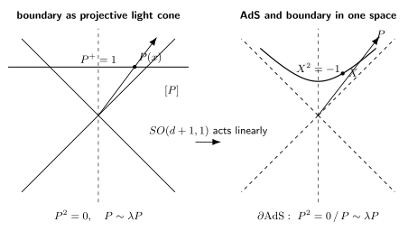
A schematic two-dimensional slice of the embedding construction. CFT boundary points are null rays $P^2=0$ modulo $P\sim\lambda P$. The gauge $P^+=1$ chooses one representative $P(x)$ of each finite boundary point. Euclidean AdS is the hyperboloid $X^2=-1$ inside the same ambient space, and its boundary is approached by $X(z,x)\sim z^{-1}P(x)$ as $z\to0$.

The basic distance identity

For two points $x_i,x_j$, write $P_i=P(x_i)$ and $P_j=P(x_j)$. Then

$$P_i\cdot P_j =-\frac12(x_i^2+x_j^2)+x_i\cdot x_j =-\frac12(x_i-x_j)^2.$$

It is therefore natural to define

$$P_{ij}\equiv -2P_i\cdot P_j.$$

On the section $P^+=1$,

$$P_{ij}=x_{ij}^2, \qquad x_{ij}^\mu=x_i^\mu-x_j^\mu.$$

This formula is the first little miracle: the ordinary squared distance is an ambient inner product.

Infinity and the compactified space

The section $P^+=1$ does not cover the whole projective cone. Null rays with $P^+=0$ are points at conformal infinity. A useful representative of the point at infinity is

$$P_\infty=(0,1,0^\mu).$$

This clarifies inversion. The origin is

$$P(0)=(1,0,0^\mu).$$

Inversion is simply the exchange

$$P^+\leftrightarrow P^-.$$

So the origin maps to $P_\infty$. Nothing singular happens on the projective cone; singularities only appear after choosing the flat section.

Linear conformal transformations

The group $SO(d+1,1)$ acts linearly on $P^A$ and preserves $P\cdot Q$. Therefore it maps null rays to null rays. After acting on $P(x)$, we return to the flat section by a projective rescaling:

$$\Lambda P(x)=\rho(x)P(x').$$

The new point $x'$ is the conformally transformed point in ordinary coordinates. The factor $\rho(x)$ is the compensating scale needed to restore the choice $P^+=1$.

For example, inversion gives

$$(1,x^2,x^\mu)\mapsto (x^2,1,x^\mu) \sim \left(1,\frac1{x^2},\frac{x^\mu}{x^2}\right),$$

so

$$x^\mu\mapsto \frac{x^\mu}{x^2}.$$

Translations are also linear upstairs:

$$P^+\mapsto P^+, \qquad P^\mu\mapsto P^\mu+a^\mu P^+, \qquad P^-\mapsto P^-+2a\cdot P+a^2P^+.$$

Applied to $P(x)$, this gives

$$P(x)\mapsto P(x+a).$$

A special conformal transformation is inversion, then translation, then inversion. In ordinary coordinates it becomes

$$x^\mu\mapsto \frac{x^\mu-b^\mu x^2}{1-2b\cdot x+b^2x^2},$$

but in embedding space it is just another linear transformation.

Sections are Weyl frames

The flat representative obeys

$$dP(x)^2=dx^2.$$

If we choose another section

$$\widehat P(x)=\Omega(x)P(x),$$

then, using $P^2=0$ and $P\cdot dP=0$,

$$d\widehat P^2=\Omega(x)^2dP^2=\Omega(x)^2dx^2.$$

Thus changing the section of the projective cone is exactly a Weyl transformation of the physical metric:

$$g_{\mu\nu}\mapsto \Omega(x)^2g_{\mu\nu}.$$

This is the geometric reason the same cone describes flat space, the cylinder $S^{d-1}\times\mathbb R$, and the sphere: they are different Weyl frames of the same conformal geometry.

Scalar primaries as homogeneous functions

A scalar primary of dimension $\Delta$ is lifted to a homogeneous function $\Phi(P)$ on the null cone:

$$\Phi(\lambda P)=\lambda^{-\Delta}\Phi(P).$$

The physical operator is obtained by pullback to the section:

$$\mathcal O(x)=\Phi(P(x)).$$

The conformal dimension is now the homogeneity degree on the projective cone. A correlator must therefore have the correct weight under independent rescalings of each point:

$$G(\lambda_1P_1,\ldots,\lambda_nP_n) = \prod_{i=1}^n \lambda_i^{-\Delta_i}G(P_1,\ldots,P_n).$$

This is often the fastest way to derive scalar correlators.

Two- and three-point functions

For two scalar primaries, the only invariant is $P_{12}$. Hence

$$\langle \Phi_1(P_1)\Phi_2(P_2)\rangle =\frac{C_{12}}{P_{12}^a}.$$

Since $P_{12}\mapsto \lambda_1\lambda_2P_{12}$, homogeneity requires

$$a=\Delta_1=\Delta_2.$$

Thus, after diagonalizing operators with identical quantum numbers,

$$\langle \Phi_i(P_1)\Phi_j(P_2)\rangle =\frac{\delta_{ij}}{P_{12}^{\Delta_i}}.$$

On the flat section,

$$\langle \mathcal O_i(x_1)\mathcal O_j(x_2)\rangle =\frac{\delta_{ij}}{(x_{12}^2)^{\Delta_i}}.$$

For three scalar primaries, write

$$\langle \Phi_1(P_1)\Phi_2(P_2)\Phi_3(P_3)\rangle = \frac{C_{123}}{P_{12}^aP_{23}^bP_{13}^c}.$$

Homogeneity gives

$$a+c=\Delta_1, \qquad a+b=\Delta_2, \qquad b+c=\Delta_3.$$

Solving,

$$a=\frac{\Delta_1+\Delta_2-\Delta_3}{2}, \qquad b=\frac{\Delta_2+\Delta_3-\Delta_1}{2}, \qquad c=\frac{\Delta_1+\Delta_3-\Delta_2}{2}.$$

Therefore

$$\boxed{ \langle \Phi_1(P_1)\Phi_2(P_2)\Phi_3(P_3)\rangle = \frac{C_{123}} {P_{12}^{\frac{\Delta_1+\Delta_2-\Delta_3}{2}} P_{23}^{\frac{\Delta_2+\Delta_3-\Delta_1}{2}} P_{13}^{\frac{\Delta_1+\Delta_3-\Delta_2}{2}}}. }$$

The coefficient $C_{123}$ is dynamical data. The powers of $P_{ij}$ are kinematics.

Four-point functions and cross-ratios

At four points, two independent cross-ratios appear:

$$u=\frac{P_{12}P_{34}}{P_{13}P_{24}}, \qquad v=\frac{P_{14}P_{23}}{P_{13}P_{24}}.$$

On the flat section,

$$u=\frac{x_{12}^2x_{34}^2}{x_{13}^2x_{24}^2}, \qquad v=\frac{x_{14}^2x_{23}^2}{x_{13}^2x_{24}^2}.$$

For identical scalar primaries of dimension $\Delta$, a common convention is

$$\langle \Phi(P_1)\Phi(P_2)\Phi(P_3)\Phi(P_4)\rangle = \frac{\mathcal G(u,v)}{P_{12}^{\Delta}P_{34}^{\Delta}}.$$

The function $\mathcal G(u,v)$ is dynamical. The OPE and crossing symmetry will constrain it later.

Spinning operators

Embedding space becomes especially useful for spinning operators. A symmetric traceless spin-$\ell$ primary can be packaged using an auxiliary polarization vector:

$$\Phi(P,Z)=Z_{A_1}\cdots Z_{A_\ell}\Phi^{A_1\cdots A_\ell}(P).$$

The conditions are

$$P^2=0, \qquad Z^2=0, \qquad P\cdot Z=0.$$

There is also the gauge redundancy

$$Z\sim Z+\alpha P.$$

The homogeneity is

$$\Phi(\lambda P,\beta Z+\gamma P) =\lambda^{-\Delta}\beta^\ell \Phi(P,Z).$$

A physical polarization $z^\mu$ is embedded by

$$Z(x,z)=z^\mu \frac{\partial P(x)}{\partial x^\mu} =(0,2x\cdot z,z^\mu).$$

Then

$$P(x)\cdot Z(x,z)=0, \qquad Z(x,z)^2=z^2.$$

Thus $z^2=0$ implements tracelessness.

Two common gauge-invariant building blocks are

$$H_{ij} =-2\left[(Z_i\cdot Z_j)(P_i\cdot P_j)-(Z_i\cdot P_j)(Z_j\cdot P_i)\right],$$

and

$$V_{i,jk} = \frac{(Z_i\cdot P_j)(P_i\cdot P_k)-(Z_i\cdot P_k)(P_i\cdot P_j)}{P_j\cdot P_k}.$$

Different references normalize these objects differently. The invariant content is the same: spinning tensor structures are homogeneous, transverse, and invariant under $Z_i\to Z_i+\alpha_iP_i$.

The AdS hyperboloid

The same ambient space contains AdS. Set the AdS radius to $1$. Euclidean $AdS_{d+1}$ is

$$X^2=-1, \qquad X^+>0.$$

A convenient Poincare-coordinate embedding is

$$X(z,x)=\frac1z(1,z^2+x^2,x^\mu), \qquad z>0.$$

It obeys $X^2=-1$. As $z\to0$,

$$X(z,x)\sim \frac1zP(x).$$

Thus the conformal boundary of AdS is the same projective null cone used to represent CFT points.

The basic bulk-boundary invariant is

$$-2P(y)\cdot X(z,x)=\frac{z^2+(x-y)^2}{z}.$$

Therefore the scalar bulk-to-boundary propagator can be written as

$$K_\Delta(X;P)=\frac{\mathcal C_\Delta}{(-2P\cdot X)^\Delta}.$$

In Poincare coordinates,

$$K_\Delta(z,x;y) =\mathcal C_\Delta\left(\frac{z}{z^2+(x-y)^2}\right)^\Delta.$$

This formula is the first concrete bridge from CFT embedding-space kinematics to AdS calculations.

AdS/CFT checkpoint

Embedding space makes three facts manifest:

$$\begin{array}{ccc} \text{CFT point} & \longleftrightarrow & P^2=0,\quad P\sim\lambda P,\\ \text{AdS point} & \longleftrightarrow & X^2=-1,\\ \text{shared symmetry} & \longleftrightarrow & SO(d+1,1)\text{ or }SO(d,2). \end{array}$$

The basic bulk-boundary invariant is $-2P\cdot X$. The basic boundary-boundary invariant is $P_{ij}=-2P_i\cdot P_j$.

How to use the formalism in practice

For scalar correlators, the recipe is almost mechanical. First write all possible ambient inner products $P_i\cdot P_j$. Then impose the correct projective weight at each point. Finally choose a section, usually $P_i=P(x_i)$, to recover the ordinary coordinate-space expression.

For spinning correlators, the same logic applies with one extra rule: every expression must be invariant under

$$Z_i\to Z_i+\alpha_iP_i.$$

This gauge redundancy removes unphysical ambient components. It is the embedding-space version of the statement that a CFT tensor lives tangent to the physical spacetime, not in the extra radial direction of the cone.

A proposed expression should pass four checks:

1. It is built from ambient contractions, so $SO(d+1,1)$ or $SO(d,2)$ covariance is manifest.
2. It has the correct homogeneity in every $P_i$.
3. It is invariant under $Z_i\to Z_i+\alpha_iP_i$ whenever polarizations are present.
4. After setting $P_i=P(x_i)$ and $Z_i=Z(x_i,z_i)$, it reduces to a sensible physical-space tensor structure.

This is why embedding space is so useful in the conformal bootstrap. Tensor structures that look painful in physical coordinates become polynomial algebra in $P_i$ and $Z_i$.

Generators in embedding space

The conformal algebra also becomes simple. On scalar ambient functions, the linear generators are

$$J_{AB}=P_A\frac{\partial}{\partial P^B}-P_B\frac{\partial}{\partial P^A}.$$

They obey the $\mathfrak{so}(d+1,1)$ algebra in Euclidean signature, or $\mathfrak{so}(d,2)$ in Lorentzian signature. The usual generators $P_\mu$, $K_\mu$, $D$, and $M_{\mu\nu}$ are linear combinations of these $J_{AB}$ after choosing lightcone coordinates $P^+$ and $P^-$. This is the algebraic reason conformal Casimir equations are cleaner in embedding notation.

One should remember, however, that the ambient function is defined only up to its values away from the cone. Physical statements must be independent of any arbitrary off-cone extension. Homogeneity and projective gauge invariance are what keep the calculation honest.

Lorentzian caution

The formulas above are algebraic. Lorentzian CFT also requires causal information: Wightman ordering, time ordering, retarded commutators, and $i\epsilon$ prescriptions. Embedding space makes $SO(d,2)$ covariance manifest, but it does not by itself choose a Lorentzian correlator. The same algebraic expression can correspond to different real-time orderings depending on how the singularities are approached.

This distinction matters in holography. Euclidean bulk-to-boundary propagators are straightforward powers of $-2P\cdot X$. Lorentzian propagators require the correct contour or $i\epsilon$ prescription, especially near light cones and horizons.

Exercises

Exercise 1: Null representative

Show that $P(x)=(1,x^2,x^\mu)$ is null and that $P_{ij}=x_{ij}^2$.

Solution

Using

$$P\cdot Q=-\frac12(P^+Q^-+P^-Q^+)+P^\mu Q_\mu,$$

we get

$$P(x)^2=-x^2+x^2=0.$$

For two points,

$$P_i\cdot P_j=-\frac12(x_i^2+x_j^2)+x_i\cdot x_j.$$

Therefore

$$-2P_i\cdot P_j=x_i^2+x_j^2-2x_i\cdot x_j=(x_i-x_j)^2.$$

Exercise 2: Inversion

Show that swapping $P^+$ and $P^-$ gives physical inversion $x^\mu\to x^\mu/x^2$.

Solution

Start from

$$P(x)=(1,x^2,x^\mu).$$

After swapping $P^+$ and $P^-$,

$$P(x)\mapsto(x^2,1,x^\mu).$$

Using projectivity,

$$(x^2,1,x^\mu)\sim \left(1,\frac1{x^2},\frac{x^\mu}{x^2}\right).$$

This is $P(x')$ with $x'^\mu=x^\mu/x^2$.

Exercise 3: Three-point exponents

Derive the scalar three-point powers from homogeneity.

Solution

Write

$$\langle\Phi_1\Phi_2\Phi_3\rangle =\frac{C_{123}}{P_{12}^aP_{23}^bP_{13}^c}.$$

Homogeneity at $P_1,P_2,P_3$ gives

$$a+c=\Delta_1, \qquad a+b=\Delta_2, \qquad b+c=\Delta_3.$$

Solving gives

$$a=\frac{\Delta_1+\Delta_2-\Delta_3}{2}, \qquad b=\frac{\Delta_2+\Delta_3-\Delta_1}{2}, \qquad c=\frac{\Delta_1+\Delta_3-\Delta_2}{2}.$$

Exercise 4: Polarization lift

Verify that $Z(x,z)=(0,2x\cdot z,z^\mu)$ satisfies $P(x)\cdot Z(x,z)=0$ and $Z(x,z)^2=z^2$.

Solution

Since $P(x)=(1,x^2,x^\mu)$,

$$P\cdot Z=-\frac12(1)(2x\cdot z)+x\cdot z=0.$$

Also,

$$Z^2=-Z^+Z^-+Z^\mu Z_\mu=z^2,$$

because $Z^+=0$.

Exercise 5: Bulk-to-boundary invariant

Show that

$$-2P(y)\cdot X(z,x)=\frac{z^2+(x-y)^2}{z}.$$

Solution

Using

$$P(y)=(1,y^2,y^\mu), \qquad X(z,x)=\frac1z(1,z^2+x^2,x^\mu),$$

we find

$$P(y)\cdot X(z,x) =-\frac12\left(\frac{z^2+x^2}{z}+\frac{y^2}{z}\right)+\frac{x\cdot y}{z}.$$

Thus

$$P(y)\cdot X(z,x) =-\frac{z^2+x^2+y^2-2x\cdot y}{2z} =-\frac{z^2+(x-y)^2}{2z}.$$

Multiplying by $-2$ gives the result.

Summary

The embedding-space dictionary is

$$x^\mu\longleftrightarrow P(x)=(1,x^2,x^\mu), \qquad P^2=0, \qquad P\sim\lambda P.$$

The basic invariant is

$$P_{ij}=-2P_i\cdot P_j=x_{ij}^2.$$

A scalar primary is a homogeneous function on the cone:

$$\Phi(\lambda P)=\lambda^{-\Delta}\Phi(P).$$

AdS is the hyperboloid $X^2=-1$ in the same ambient space, and its boundary is the same projective null cone. This is why embedding space is one of the cleanest bridges from CFT kinematics to the AdS/CFT dictionary.