Introduction

renphysics

To be completed

A slogan of AdS/CFT is bulk quantum gravity = boundary QFT, or sometimes GR = RG. Before digging into the AdS/CFT, let us start with known basic laws of nature and their limitations.

1. Black hole entropy

Black hole thermodynamics shows that entropy scales with horizon area rather than volume, linking gravity, relativity, quantum mechanics, and statistical physics. This area law implies an upper bound on information set by the boundary of a region, motivating the holographic principle that a gravitating system’s degrees of freedom can be encoded on a lower‑dimensional boundary.

A quantum theory of gravity in a region is equivalent to a non-gravitational quantum theory living on the boundary of that region.

This violates everyday intuition because everyday intuition is based on nearly flat spacetime, where one can pack information into a volume. But when the energy density becomes large enough, gravitational effects can no longer be neglected and black hole formation becomes relevant. Then the area law becomes the correct statement about maximal entropy. Roughly speaking, one can heuristically say “about one bit per Planck area”, up to the factor of $1/4$.

In this remarkable formula

• $\hbar$: quantum physics,
• $c$: relativity,
• $k_B$: statistical physics / thermodynamics,
• $G$: gravity,
• and a geometric quantity: area.

2. Symmetries

Symmetries play a crucial role in modern theoretical physics. Before Einstein, symmetry was often viewed as something we discovered after we knew the laws: first we propose a physical law, then we ask what symmetries it possesses. For instance, Newtonian mechanics is invariant under Galilean transformations (Galilean invariance); Maxwell’s equations are invariant under Lorentz transformations (Lorentz invariance) and, crucially, under gauge transformations (gauge invariance). Historically, Maxwell himself did not formulate his equations by first declaring “Lorentz invariance” as a principle; that viewpoint came later. One can even say that Einstein, in 1905, extracted the principle of Lorentz invariance from Maxwell’s theory and elevated it to the status of a fundamental postulate of physics.

After Einstein, symmetry was gradually elevated to a new level: it became closer to a “first principle.” Namely:

• We propose a symmetry principle.
• We ask: what is the most general form of physical laws consistent with this symmetry?
• Then we check whether nature realizes such laws.

In modern field theory, many Lagrangians can be thought of as being fixed (to a very large extent) by: symmetry requirements (spacetime symmetries and internal/gauge symmetries), plus a derivative expansion (keeping terms with up to a certain number of derivatives, typically up to two derivatives for a “minimal” renormalizable theory in four dimensions). This severely restricts the possible terms. Using this kind of principle, we can write down the Lagrangians for various fields and then combine them.

In fact, one can write essentially the whole structure—general relativity plus the Standard Model—in a compact “one-line” form using the Feynman path integral, including gauge fields, fermions, Yukawa couplings, scalar potentials, and so on. Schematically:

Adapted from a slide by Neil Turok.

Noether's theorems

Noether’s original 1918 paper Invariante Variationsprobleme (“Invariant Variation Problems”) English translation.

Noether’s (first) theorem: global symmetries → conserved charges that generate physical symmetry transformations.

Noether’s second theorem: local/gauge symmetries → differential identities among the Euler–Lagrange equations (“Noether identities”), which in Hamiltonian language show up as first-class constraints (gauge redundancy).

Historical note: Noether did not present them as two disconnected ideas; rather, she treated them as two branches of one general “invariant variational problem,” depending on whether the symmetry group is parameterized by constants (finite-dimensional) or by arbitrary functions (infinite-dimensional).

Symmetries in Minkowski spacetime

Suppose I have an object moving in (say) a two-dimensional Euclidean plane. The essence of Euclidean geometry is the invariance of the distance. For example, $ds^2 = dx^2 + dy^2$, or in finite form, $\ell^2 = (\Delta x)^2 + (\Delta y)^2$. Transformations that preserve this length are translations in two directions plus rotations—altogether three independent isometries.

In special relativity the invariant “length” in four-dimensional Minkowski spacetime is

$$ds^2 = -c^2 dt^2 + dx^2 + dy^2 + dz^2.$$

The transformations that preserve this interval gives the Poincaré group, which has 10 generators: 6 Lorentz transformations plus 4 translations. The greatness of special relativity is not simply “what becomes relative”. It is also about what remains absolute. The absolute (invariant) quantities reveal the essence of the problem.

A very beautiful fact is that the Poincaré group has (essentially) two independent Casimir invariants, which correspond to mass and spin. In other words, a particle (or, equivalently, a field) can be labeled by an irreducible representation of the Poincaré group, characterized by its mass and spin.

A further refinement is to push symmetry principles to an extreme by extending spacetime symmetry to supersymmetry, a symmetry between bosons and fermions. Supersymmetry plays an important role in the consistency of superstring theory.

Fields in the Standard Model and symmetry as a guiding principle

In the Standard Model, the basic particles/fields can be classified by spin:

• Spin $1/2$: spinor fields (matter fermions).
• Spin $1$: gauge fields (electromagnetic, weak, and strong interactions).
• Spin $0$: scalar fields (e.g. the Higgs).
• Spin $2$: the gravitational field (the metric).

To describe these fields we need a Lagrangian (or action). The guiding principle is symmetry.

For fun: New year wishes from great physicists

• Newton
• Maxwell
• Dirac
• Hawking

3. From special relativity to general relativity

Why must special relativity be generalized to general relativity?

The basic reason is simple: Newton’s law of gravitation is incompatible with special relativity.

Newtonian gravity has instantaneous action at a distance: place two masses somewhere, and they exert gravitational force on each other “immediately”. But in special relativity, for one particle to influence another, information must propagate causally at finite speed. In gravity, that causal influence is carried by gravitational waves.

Reconciling these ideas is highly nontrivial. Einstein spent about ten years to complete it.

For comparison: Coulomb’s law also looks instantaneous, but its consistent relativistic completion is Maxwell’s theory, which automatically contains Lorentz invariance (as mentioned above). For gravity the completion is general relativity.

The equivalence principle and general covariance

A key idea is the equivalence principle: the effects of acceleration and gravity are locally equivalent.

General relativity is beautifully summarized by the idea that the laws of physics should be formulated in a way that is valid for all observers, regardless of their state of motion, including acceleration. A common slogan is that general relativity is “generally covariant”.

Spacetime tells matter how to move; matter tells spacetime how to curve. —John Wheeler

Einstein’s equation

The basic equation of general relativity is Einstein’s equation,

$$G_{\mu\nu} + \Lambda g_{\mu\nu} = 8\pi G\,T_{\mu\nu}, \qquad G_{\mu\nu} \equiv R_{\mu\nu}-\frac{1}{2}R\,g_{\mu\nu}.$$

Solving Einstein’s equation means determining the spacetime geometry—how to measure lengths and times.

Let me emphasize something that is important both conceptually and technically: when solving Einstein’s equation, one often uses coordinate freedom (diffeomorphism invariance) to choose a gauge. For example, even in two dimensions, a generic metric can be written with several functions, but because all 2D metrics are locally conformally flat, there is large coordinate freedom to simplify the form. This is essentially “choosing a gauge”.

I think an exact solution of Einstein’s equation is like an ancient poem: concise and elegant, using very few symbols to express rich meaning. A common feature is that such solutions usually have high symmetry.

However, the relation between symmetry and difficulty differs between poetry and gravity:

• For poetry, stronger symmetry constraints generally make it harder to write.
• For exact solutions of Einstein’s equation, stronger symmetry typically makes it easier to find solutions, because the spacetime becomes simpler.

One can “lower” symmetry step by step to obtain more general spacetimes—for instance, from spherical symmetry to cylindrical symmetry, then to axisymmetry, etc.

The Schwarzschild solution and the global structure

The first exact solution of Einstein’s equation is the Schwarzschild solution, found essentially in 1916, almost at the same time when Einstein finished general relativity. Remarkably, Schwarzschild found it while serving on the front lines of World War I. Although the solution was written down early, it took decades (roughly the 1950s–60s) for the community to fully understand that it describes a black hole.

In standard coordinates (setting $c=1$ for simplicity) the Schwarzschild metric is

$$ds^2 = -\left(1-\frac{2GM}{r}\right)dt^2 + \left(1-\frac{2GM}{r}\right)^{-1}dr^2 + r^2 d\Omega_2^2 .$$

The key point is that a coordinate chart does not necessarily cover the entire spacetime. The usual Schwarzschild coordinates only cover part of the maximally extended geometry. The full extension contains regions interpreted as the exterior black hole region, the black hole interior, as well as a white hole region and another asymptotic region (another “universe”) in the idealized maximal extension.

• Crossing the horizon and the equivalence principle: If you are freely falling in a spaceship toward the horizon, the moment you cross the horizon (the “point of no return”) you do not feel anything special locally. This is the equivalence principle at work: locally, in free fall, gravity can be “transformed away”, much as an astronaut in deep space experiences weightlessness.

• Hawking radiation: black holes are not completely black: After understanding the classical black hole solution, a major discovery by Hawking is that black holes are not entirely black: they emit thermal radiation. A very intuitive picture is that quantum fluctuations can create particle–antiparticle pairs near the horizon. If one particle falls into the black hole while the other escapes to infinity, the escaping particle appears as radiation emitted by the black hole. The Hawking temperature is

  $$T_H = \frac{\hbar c^3}{8\pi G k_B M},$$

  so for a black hole of one solar mass it is extremely small (of order $10^{-6}\,\mathrm{K}$ in this talk’s rough estimate), much lower than the cosmic microwave background temperature. This is why Hawking radiation is very hard to observe directly for astrophysical black holes.

4. Quantum field theory, scales, and universality

A quantum field theory differs from a classical theory because of quantum fluctuations. A basic question is: how large are quantum effects?

In some theories (e.g. QED), the low-energy limit is close to a classical field equation (Maxwell’s equations), so quantum effects can be small in many situations. In other theories, especially non-abelian gauge theories at low energy, quantum effects cannot be ignored.

This brings in the idea of an energy scale.

7.1 UV vs IR: small scales vs large scales

It is useful to compare two ways of looking at a complex object:

• At very small scales, things look messy and complicated.
• At large scales, after “coarse-graining” (discarding microscopic details), simple patterns and laws may emerge.

We often use “UV” (ultraviolet) to mean high energy / short distance, and “IR” (infrared) to mean low energy / long distance.

A rough scaling is

$$E \sim \frac{\hbar c}{\ell}.$$

For example, the hydrogen atom has a radius of order the Bohr radius, and the energy needed to ionize it is of order eV. If you probe physics at distances smaller by several orders of magnitude, you must inject energies larger by the corresponding orders of magnitude.

7.2 Universality near second-order phase transitions

Water, CO$_2$, and magnets look completely different microscopically, but they can share the same underlying universal behavior near a second-order phase transition. The key concept is the correlation length $\xi$:

• If $\xi$ is finite and small, a local perturbation only affects a few nearby atoms.
• Near a critical point, $\xi$ can become very large (in the ideal limit, $\xi\to\infty$). Then the system has long-range correlations and can often be described by a relatively simple effective field theory.

This is why such systems can fall into the same universality class, even though they are microscopically different.

Renormalizability and why quantizing gravity is hard

Let me now look at the four fundamental interactions from the perspective of quantum field theory.

In perturbation theory, interactions arise from exchanging quanta (bosons). A typical process has a tree-level diagram (single exchange) and loop corrections (multiple exchanges). If loop contributions become comparable to tree-level contributions, quantum effects are strong and cannot be neglected.

A very general diagnostic is the mass dimension of the coupling constant.

Dimensional analysis of couplings

Suppose a coupling $g$ has mass/energy dimension

$$[g] = E^{\alpha}.$$

Then:

$$\frac{A_1}{A_0}\sim\kappa^2E^{-2\alpha},\qquad \frac{A_2}{A_0}\sim\kappa^4\int dE' E'^{-4\alpha-1}$$

• If $\alpha>0$, the theory is typically super-renormalizable (UV behavior improves).
• If $\alpha=0$, the theory is renormalizable (UV behavior is marginal and needs detailed beta-function analysis).
• If $\alpha<0$, the theory is non-renormalizable in perturbation theory (UV behavior worsens).

In four spacetime dimensions, Yang–Mills gauge couplings are dimensionless ($\alpha=0$), while Newton’s constant has

$$[G] = E^{-2}.$$

Equivalently, the gravitational coupling $\kappa\sim\sqrt{G}$ has

$$[\kappa] = E^{-1}.$$

This already hints that perturbative quantum gravity becomes strongly coupled at high energies.

The Planck scale

A standard estimate is that quantum gravity becomes important around the Planck energy

$$M_P \sim \frac{1}{\sqrt{G}} \sim 10^{19}\ \mathrm{GeV},$$

where (roughly) loop effects become order one.

From the loop-integral viewpoint: in a loop diagram one integrates over unconstrained high momenta. With negative mass dimension coupling, divergences typically become worse at higher energy, signaling non-renormalizability.

This is why constructing a UV-complete quantum theory of gravity is so challenging.

At the same time, note the complementary fact: although gravity is problematic in the UV, its IR (low-energy) behavior is extremely well described by classical general relativity. In contrast, some condensed matter systems can be UV-benign but flow to strongly coupled behavior in the IR (e.g. to an interacting conformal fixed point), where perturbation theory fails.

5. IR and UV Properties of Fundamental Interactions

Conventions. Natural units ($\hbar=c=1$). “Coupling mass dimension” means the energy (mass) dimension of the interaction strength. Spacetime dimension is $d=4$ unless noted; the last row is $d=3$.

Interaction	Coupling mass dimension	IR / low energy / large scales	UV / high energy / short scales
Gravity (GR)	$E^{-1}$ for $\kappa=\sqrt{32\pi G_N}$; $[G_N]=E^{-2}$	Einstein field equations; EFT expansion in $E/M_{\mathrm{Pl}}$	Perturbatively nonrenormalizable; dimensionless $g(\mu)\sim \mu^2 G_N$ grows; needs UV completion
Electromagnetism (QED)	$E^0$ for $e$; $\alpha=e^2/4\pi$	Maxwell equations; long‑range $1/r^2$; IR divergences cancel in inclusive rates	Renormalizable; $\beta(\alpha)>0$ (screening); Landau pole at exponentially high $\mu$
Weak interaction	$E^{-2}$ for Fermi $G_F$ (IR EFT); $E^0$ for SM $g,g'$ (UV completion)	Fermi 4‑fermion EFT; nonrenormalizable; valid for $\mu\ll m_W$	Renormalizable $SU(2)_L\times U(1)_Y$ gauge theory; spontaneous breaking; massive $W^\pm,Z$
Strong interaction (QCD)	$E^0$ for $g_s$; $\alpha_s=g_s^2/4\pi$	Strong coupling; confinement; chiral symmetry breaking; hadrons as IR dof	Asymptotic freedom; $\alpha_s(\mu)\to 0$ as $\mu\to\infty$; perturbative at high $\mu$
$\lambda\phi^4$ in $d=3$	$E^{+1}$ for $\lambda$	Interacting IR fixed point (Wilson–Fisher CFT); e.g. $N{=}1$ $\to$ 3D Ising	Super‑renormalizable; Gaussian UV fixed point; $\tilde\lambda(\mu)=\lambda/\mu\to 0$

Brief explanations

• IR vs. UV. “IR/low energy/large scales” refers to physics at momenta $\mu$ much smaller than the relevant heavy scales; “UV/high energy/small scales” refers to $\mu$ large compared to those scales.

• Terminology.

  • Renormalizable: finitely many parameters absorb all divergences to all loop orders (e.g., QED, QCD, electroweak).
  • Nonrenormalizable (as EFT): infinite tower of higher‑dimension operators suppressed by a cutoff; predictive in a low‑energy expansion (e.g., gravity, Fermi theory).
  • Super‑renormalizable: only a finite set of divergent structures; UV controlled by the Gaussian fixed point (e.g., $\phi^4$ in $d=3$).

• Gravity as an EFT. The loop expansion is organized by operators suppressed by $M_{\mathrm{Pl}}$. The dimensionless strength $g(\mu)\sim \mu^2 G_N$ increases with $\mu$, so the EFT breaks near $M_{\mathrm{Pl}}$ and requires a UV completion (e.g., asymptotic safety or string theory, model‑dependent).

• QED running and the Landau pole. One‑loop running:

  $$\frac{d\alpha}{d\ln\mu}=\frac{2N_f}{3\pi}\alpha^2+\cdots>0$$

  Screening implies $\alpha(\mu)$ grows logarithmically and formally hits a Landau pole at an exponentially high scale, so QED is best viewed as an EFT embedded in the full Standard Model.

• QCD asymptotic freedom. One‑loop running:

  $$\frac{d\alpha_s}{d\ln\mu}=-\frac{11-\tfrac{2}{3}N_f}{2\pi}\alpha_s^2+\cdots<0\quad (N_f\lesssim 16)$$

  Antiscreening by gluons drives $\alpha_s(\mu)\to 0$ at large $\mu$; in the IR, confinement and a mass gap dominate the dynamics.

• Weak interaction: IR EFT vs. UV completion.

  • Low energies: Fermi theory with coupling $G_F$ (dimension $E^{-2}$), a nonrenormalizable contact interaction valid for $\mu\ll m_W$.
  • Matching relation: $G_F/\sqrt{2}=g^2/(8m_W^2)$.
  • High energies: renormalizable electroweak theory $SU(2)_L\times U(1)_Y$ with dimensionless $g,g'$, spontaneously broken to electromagnetism; $W^\pm,Z$ acquire masses.

• $\phi^4$ in $d=3$ and the Wilson–Fisher fixed point. Writing a dimensionless coupling $\tilde\lambda(\mu)=\lambda/\mu$, the $\beta$‑function near $d=4-\varepsilon$ has the schematic form

  $$\beta(\tilde\lambda)=-\varepsilon\,\tilde\lambda+c\,\tilde\lambda^2+\cdots,\quad c>0,$$

  giving an interacting IR fixed point at $\tilde\lambda_\ast\sim \varepsilon/c$ (set $\varepsilon=1$ for $d=3$). The theory is super‑renormalizable with finitely many primitive divergences.

---

A Chinese traditional poem by C.N. Yang

赞陈氏级 (In Praise of Chern Class) --- C.N. Yang

天衣岂无缝，(Can Heaven’s robe truly be without seams?)
匠心剪接成。(By a master’s craft it is cut and joined.)
浑然归一体，(It merges back into one seamless whole—)
广邃妙绝伦。(Vast and profound, wondrous beyond compare.)
造化爱几何，(Creation itself delights in geometry;)
四力纤维能。(Fiber-bundle theory captures the four forces.)
千古寸心事，(A matter for a thousand ages, known to the inch-heart:)
欧高黎嘉陈。(Euclid, Gauss, Riemann, Cartan—and Chern.)

The last two lines encode a thread: these mathematicians pushed geometry forward by generalizing the Euclidean statement that the sum of angles in a triangle is $180^\circ$. Each step is a deeper generalization of geometry, and the development of differential geometry moved forward accordingly. Their major contributions are: Euclid (Euclidean geometry), Gauss (intrinsic geometry and curvature of surfaces), Riemann (higher-dimensional curved manifolds), Cartan (moving frames, differential forms), Chern (connections, characteristic classes).

---

5. Motivation for strings

5.1 Motivation from quantum gravity (UV completion)

For the electromagnetic field (and more generally gauge fields), the action can be written elegantly using differential forms:

$$S_{\text{gauge}} = -\frac{1}{2g^2}\int \mathrm{tr}(F\wedge \star F),$$

where $F$ is the curvature 2-form of a connection $A$ (in components, $F_{\mu\nu}=\partial_\mu A_\nu-\partial_\nu A_\mu$ for the Abelian case, and $F_{\mu\nu}^a$ with commutator terms for the non-Abelian case). Yang and Mills’ contribution can be viewed geometrically: they promoted the gauge potential from an Abelian connection to a matrix-valued connection, leading to non-Abelian gauge symmetry. For gravity, the Einstein–Hilbert action is

$$S_{\text{GR}} = \frac{1}{16\pi G}\int d^4x\sqrt{-g}\,R,$$

where (R) is the Ricci scalar curvature. So there is a striking similarity between gauge theory and gravity: both are expressed in terms of curvature. This similarity is one reason Einstein was willing to devote much of his later life to a unification attempt. But the crucial difference is also clear:

• Gauge theories like electromagnetism and Yang–Mills theory can be renormalizable.
• Gravity, in the Einstein–Hilbert form, is not renormalizable.

Now, since gravity is non-renormalizable, a natural idea is: can we improve its ultraviolet behavior by adding higher-curvature terms? For instance, we could consider adding terms like

$$R^2,\qquad R_{\mu\nu}R^{\mu\nu},\qquad R_{\mu\nu\rho\sigma}R^{\mu\nu\rho\sigma}.$$

Such terms are expected to be tiny at low energies and become important only at very high energies. And indeed, higher derivatives improve ultraviolet behavior: roughly speaking, more derivatives in the kinetic operator suppress high-momentum propagators and reduce the degree of divergence of loop integrals.

But this comes at a terrible cost. Higher-derivative gravity typically introduces ghost-like states—states with negative norm (or negative kinetic energy). This violates unitarity: time evolution would not be reversible in the quantum-mechanical sense, and negative-norm states are unacceptable in a consistent quantum theory.

There is a possible “rescue strategy”: do not add just one higher-derivative term, but add infinitely many higher-derivative terms arranged so that the dangerous ghost modes cancel or are eliminated. Then one effectively replaces a finite-order differential operator with an infinite-order one, schematically something like

$$\text{(kinetic operator)} \sim \Box,f(\Box),$$

where $f(\Box)$ is an entire function expanded in infinitely many derivatives.

At an intuitive level, this has an important consequence: derivatives are local operators acting at a point, but an infinite sum of derivatives can behave like a nonlocal operator, related to an integral kernel that “smears” interactions over a region. The price for taming ultraviolet divergences is that the fundamental interaction becomes less pointlike and more extended.

This intuition is exactly what one expects if the fundamental objects are not point particles but extended objects: strings. Of course, string theory was not historically derived in precisely this way, but this line of reasoning provides a conceptual motivation for why “extendedness” can help.

In physics, the symmetry principle plays a similar role. It is natural to try to push symmetry to its extreme. In superstring theory, this is done by extending spacetime symmetries to supersymmetry, a symmetry exchanging bosons and fermions. Supersymmetry is crucial for the self-consistency of superstring theory.

5.2 Motivation from strong interactions (flux tubes)

The same phenomenon can admit two different descriptions—a kind of duality. In electromagnetism, Maxwell favored the field description: the field is fundamental, defined at each point in space. Faraday preferred the picture of lines of force. For electromagnetism, the field description is often more convenient because the field lines spread throughout space. For the strong interaction, the situation is different. Consider two quarks separated by a large distance. The color flux does not spread out like electric field lines. Instead, it becomes confined into a narrow tube connecting the quarks. In a small region, this looks like a string stretched between them. So when the interaction is weak, the point-particle description is often simplest. But when the interaction is strong, the stringlike flux tube can be a more natural effective degree of freedom. This gives another reason why strings appear naturally in the physics of strong coupling.

The anti-de Sitter/conformal field theory correspondence uses precisely this string-based viewpoint.

At weak coupling, a point-particle description (fields) is natural. At strong coupling, a string-like description may become simpler.

---

6. Introduction to AdS/CFT (Gauge/Gravity Duality)

The AdS/CFT correspondence—also called gauge/gravity duality or holographic duality—is the claim that certain quantum theories of gravity are exactly equivalent to ordinary (non-gravitational) quantum field theories. The best-understood case equates a gravitational theory on an asymptotically Anti–de Sitter spacetime in $(d{+}1)$ dimensions with a conformal field theory (CFT) in $d$ dimensions living on the AdS boundary. “Equivalent” means: the two theories have the same Hilbert space (up to a precise map), the same observables (translated through a dictionary), and the same dynamics.

What is AdS geometrically?

AdS (anti–de Sitter) is the maximally symmetric solution of Einstein’s equation with a negative cosmological constant $\Lambda<0$. Geometrically, it is the Lorentzian analogue of hyperbolic space, i.e. a spacetime of constant negative curvature.

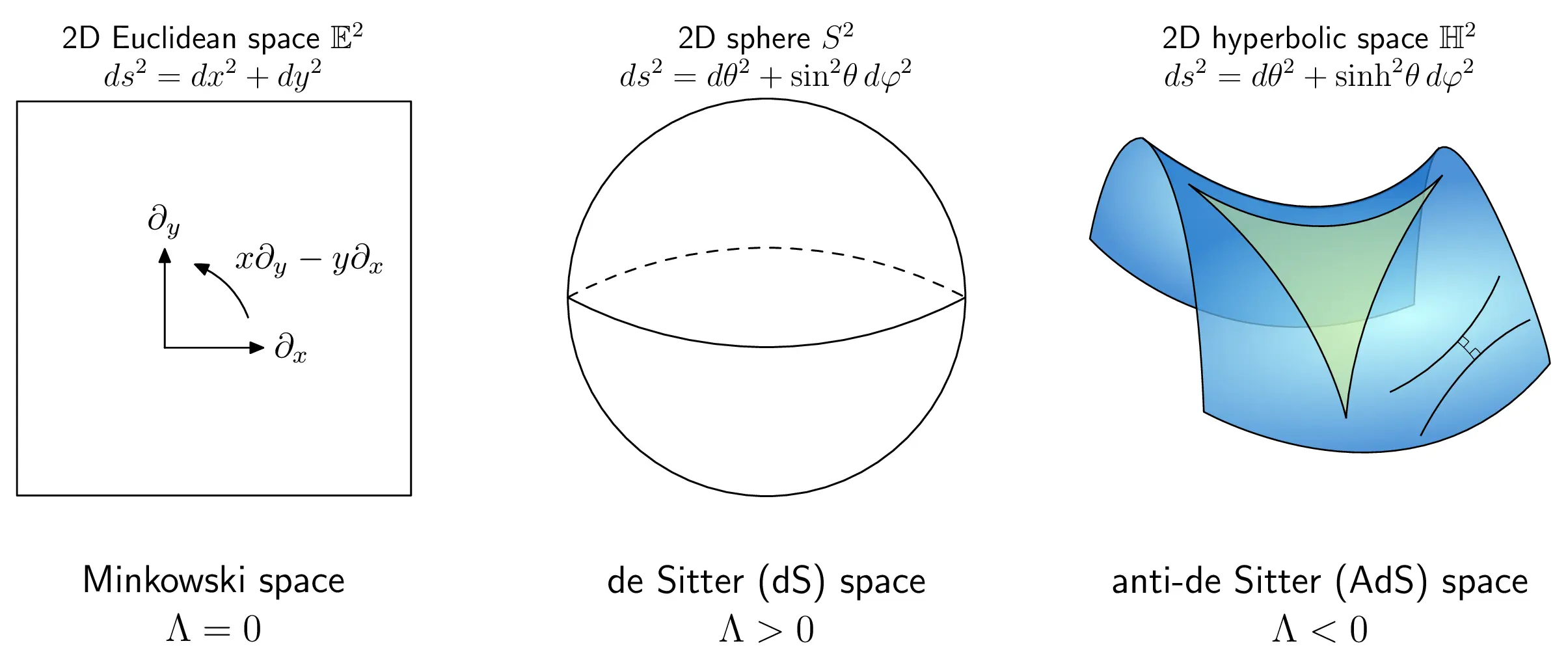
Historically, hyperbolic geometry arises when one modifies Euclid’s fifth postulate (the parallel postulate), leading to non-Euclidean geometries (Lobachevsky, Bolyai, etc.). In physics, one similarly encounters three maximally symmetric spacetimes distinguished by the sign of $\Lambda$:

• $\Lambda=0$: Minkowski spacetime (flat).
• $\Lambda>0$: de Sitter spacetime (positive curvature).
• $\Lambda<0$: anti–de Sitter spacetime (negative curvature).

One can visualize hyperbolic geometry via models such as the Poincaré disk: an infinite hyperbolic space can be mapped into a finite disk where distances become more and more “compressed” near the boundary.

Artists like M. C. Escher created famous drawings that vividly capture such hyperbolic tessellations.

A key physical interpretation in holography is that the extra (radial) direction in AdS corresponds to the energy scale of the boundary theory: moving from the boundary into the bulk is like flowing from UV to IR under the renormalization group.

---

A mathematical analogy

A complicated problem can sometimes be translated into a simpler problem by a boundary–bulk correspondence.

The fundamental theorem of calculus (Newton–Leibniz) says

$$\int_a^b f(x)\,dx = F(b)+(-1)\cdot F(a), \qquad (F' = f).$$

The left-hand side depends on the detailed behavior of $f(x)$ throughout a 1D interval. The right-hand side only depends on the values of the antiderivative at the 0D boundary points $a$ and $b$.

Stokes’ theorem, Gauss’ theorem, and many other integral identities are higher-dimensional generalizations. In the language of differential forms they can all be written in one compact formula:

$$\int_{\mathcal{M}} d\omega = \int_{\partial\mathcal{M}} \omega.$$

This equation captures precisely the relationship between a region $\mathcal{M}$ and its boundary $\partial\mathcal{M}$.

---

1) The statement (what the correspondence says)

Let $\text{AdS}_{d+1}$ denote Anti–de Sitter space of radius $L$, and let $\text{CFT}_d$ be a $d$‑dimensional conformal field theory. AdS/CFT asserts an equivalence between:

• a gravitational/string theory in the bulk (asymptotically $\text{AdS}_{d+1}$), and
• a QFT without dynamical gravity on the boundary (a $\text{CFT}_d$).

The sharpest operational statement is the equality of generating functionals (GKPW):

$$Z_{\text{bulk}}\!\left[\phi_0\right] = Z_{\text{CFT}}\!\left[J=\phi_0\right] = \Big\langle \exp\!\Big(\int d^d x\, \phi_0(x)\, \mathcal O(x)\Big)\Big\rangle_{\text{CFT}} .$$

Here $\phi_0(x)$ is the boundary value of a bulk field $\phi(x,z)$ (with $z$ the AdS radial coordinate), and $\mathcal O(x)$ is the corresponding boundary operator. Functional derivatives with respect to $\phi_0$ generate CFT correlation functions of $\mathcal O$.

What makes AdS/CFT profound is that it provides a nonperturbative definition of quantum gravity in spacetimes with AdS asymptotics, and a practical tool for computing strongly coupled QFT observables using classical gravity.

A prototypical example (the original “top-down” case) is:

$$\text{Type IIB string theory on } \text{AdS}_5 \times S^5 \quad \longleftrightarrow \quad \mathcal N=4\ \text{SYM in } d=4 \text{ with gauge group } SU(N).$$

---

2) Why should such a correspondence exist?

AdS/CFT is the confluence of three robust ideas:

2.1 Symmetry matching: isometries of AdS = conformal symmetries of the boundary

The isometry group of $\text{AdS}_{d+1}$ is $SO(d,2)$, which is exactly the conformal group of a $d$‑dimensional CFT. This makes it plausible that a bulk theory on AdS can be reorganized as a CFT living on the conformal boundary.

In Poincaré coordinates, the AdS metric can be written as

$$ds^2=\frac{L^2}{z^2}\left(dz^2+\eta_{\mu\nu}dx^\mu dx^\nu\right), \qquad z>0,$$

where the boundary is at $z\to 0$. The scaling transformation

$$x^\mu \to \lambda x^\mu,\qquad z \to \lambda z$$

is an isometry of this metric. This immediately suggests the central holographic idea:

• the radial direction $z$ geometrizes the renormalization group (RG) scale of the boundary theory.

Small $z$ corresponds to UV physics; large $z$ corresponds to IR physics. This “RG-as-geometry” principle is one of the clearest reasons the correspondence is natural.

2.2 The brane construction: one system, two low-energy descriptions

The deeper reason is that open strings and closed strings are not independent sectors in string theory: the same underlying theory admits dual descriptions where the fundamental degrees of freedom look like gauge fields (open strings) or gravity (closed strings). AdS/CFT is a particularly sharp realization of this open/closed string duality. The most concrete derivation comes from D‑branes. Consider a stack of $N$ coincident D3‑branes in type IIB string theory.

There are two standard low-energy descriptions:

(A) Open-string / gauge-theory description.
Low-energy open strings ending on the branes give a $3{+}1$‑dimensional gauge theory on the brane worldvolume: $\mathcal N=4$ super Yang–Mills with gauge group $SU(N)$.

(B) Closed-string / gravity description.
The same D3‑branes gravitate; in the closed-string description they are a classical source producing a curved spacetime. The D3‑brane solution has a “throat” region whose near-horizon geometry is $\text{AdS}_5 \times S^5$.

Now take the decoupling limit: focus on low energies as seen by an observer near the branes. In this limit, the physics splits into two decoupled sectors:

• the brane-localized gauge theory (from open strings), and
• closed strings in the near-horizon throat geometry.

Because these are two descriptions of the same underlying brane system, consistency forces them to be equivalent. That equivalence is the AdS/CFT correspondence.

2.3 Why gravity becomes classical: large $N$ and strong coupling

The duality becomes most useful in a regime where the bulk is well approximated by classical gravity. Two conditions are typical:

• Large $N$ suppresses bulk quantum loops:

  • the boundary $1/N$ expansion corresponds to the bulk genus (string loop) expansion;
  • at $N\to\infty$, the bulk is effectively classical.

• Large ’t Hooft coupling $\lambda=g_{\text{YM}}^2 N$ suppresses stringy corrections:

  • curvature in string units becomes small when $\lambda \gg 1$;
  • the bulk reduces to supergravity (plus controlled corrections).

This is the origin of the celebrated strong/weak nature: strongly coupled large-$N$ gauge theory can be computed from weakly curved classical gravity.

---

3) The core dictionary (see more)

3.1 Fields and operators

Bulk fields correspond to boundary operators:

• a bulk scalar $\phi$ $\leftrightarrow$ a scalar operator $\mathcal O$,
• a bulk gauge field $A_M$ $\leftrightarrow$ a conserved current $J^\mu$,
• the bulk metric $g_{MN}$ $\leftrightarrow$ the stress tensor $T_{\mu\nu}$.

For a scalar in $\text{AdS}_{d+1}$, the operator dimension $\Delta$ is related to the bulk mass $m$ by

$$m^2 L^2 = \Delta(\Delta-d).$$

Near the boundary, solutions behave as

$$\phi(x,z)\sim z^{d-\Delta}\,\phi_0(x) + z^{\Delta}\,A(x),$$

where $\phi_0(x)$ sources $\mathcal O(x)$ and (after holographic renormalization) $A(x)$ encodes $\langle \mathcal O(x)\rangle$.

3.2 Correlators from the bulk (GKPW in practice)

Once $Z_{\text{bulk}}[\phi_0]$ is known (often by evaluating an on-shell action), CFT correlators follow by functional differentiation. For example,

$$\langle \mathcal O(x)\rangle = \frac{\delta \ln Z_{\text{CFT}}}{\delta \phi_0(x)} = \frac{\delta \ln Z_{\text{bulk}}}{\delta \phi_0(x)} .$$

Higher-point functions are obtained by further derivatives.

3.3 Thermal states and black holes

A thermal state of the boundary theory at temperature $T$ is dual to a bulk geometry with a horizon. The simplest case is an AdS–Schwarzschild black hole, whose Hawking temperature equals the boundary temperature. Thermodynamic quantities map accordingly:

• boundary energy/pressure $\leftrightarrow$ asymptotic data of the bulk metric,
• boundary entropy density $s$ $\leftrightarrow$ horizon area via $S_{\text{BH}}=\frac{\text{Area}}{4G_N}$.

3.4 Entanglement entropy and geometry

For holographic CFTs in appropriate semiclassical regimes, the entanglement entropy of a spatial region $A$ is given by the Ryu–Takayanagi prescription:

$$S_A=\frac{\text{Area}(\gamma_A)}{4G_N},$$

where $\gamma_A$ is a bulk extremal surface anchored on $\partial A$ (and homologous to $A$). This is one of the sharpest bridges between quantum information and spacetime geometry.

Many nontrivial inequalities in quantum information theory—such as strong subadditivity—become transparent geometrically in the bulk Tensor-network pictures also give an intuitive way to visualize how boundary entanglement patterns build up a bulk geometry.

---

4) Brief summary of AdS/CFT

• AdS/CFT is an equivalence between a bulk gravitational theory on $\text{AdS}_{d+1}$ and a boundary $\text{CFT}_d$.
• It exists because the same D‑brane system has two consistent low-energy descriptions (open strings $\Rightarrow$ gauge theory, closed strings $\Rightarrow$ gravity), and because open/closed string duality demands they match.
• The radial direction is the energy scale: $z\leftrightarrow$ RG.
• Large $N$ and large $\lambda$ are the regime where classical gravity becomes a powerful computational tool.

What it is good for

• A nonperturbative definition of AdS quantum gravity.
• Black holes and information: thermalization, entropy, and microscopic unitarity in a controlled setting.
• Strong coupling: transport, hydrodynamics, and real-time dynamics in strongly coupled QFTs.
• Quantum information in QFT: entanglement structure geometrized in the bulk.

What it is not (by itself)

• A proof that our Universe is holographic (our cosmological constant is positive, not AdS).
• A guarantee that every QFT has a simple gravitational dual.
• A replacement for field theory methods at finite $N$ or weak coupling (where the bulk becomes stringy or strongly quantum).

---

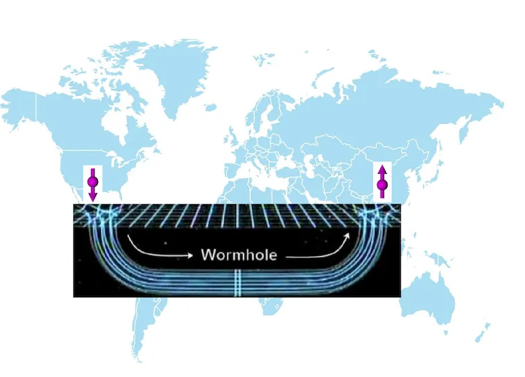
ER=EPR

• Einstein–Rosen bridge (Wormhole)
• Einstein–Podolsky–Rosen (EPR) entanglement: two entangled particles can show strong correlations even when separated by large distances.

The conjecture (due to Maldacena and Susskind) is that entanglement and wormholes are two descriptions of the same underlying connection: any two sufficiently entangled systems might be connected by a (possibly highly quantum) wormhole. This idea is deeply connected to black hole information and to the understanding of Hawking radiation, where the emitted quantum is entangled with the part that falls behind the horizon.

The entangled spins: I feel you near me even when we are apart.

Further reading

• Read AdS/CFT courses & lecture series